41 how to change excel chart data labels to custom values
How to add and customize chart data labels - Get Digital Help Double press with left mouse button on with left mouse button on a data label series to open the settings pane. Go to tab "Label Options" see image to the right. The checkboxes let you select what values you want to use as data labels. Value from cells - Lets you select a cell range that contains the values you want to use. Is there a way to change the order of Data Labels? Please try to double click the the part of the label value, and choose the one you want to show to change the order. Thanks, Rena ----------------------- * Beware of scammers posting fake support numbers here. * Once complete conversation about this topic, kindly Mark and Vote any replies to benefit others reading this thread. Report abuse
Dynamically Label Excel Chart Series Lines • My Online ... Sep 26, 2017 · To modify the axis so the Year and Month labels are nested; right-click the chart > Select Data > Edit the Horizontal (category) Axis Labels > change the ‘Axis label range’ to include column A. Step 2: Clever Formula. The Label Series Data contains a formula that only returns the value for the last row of data.

How to change excel chart data labels to custom values
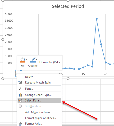
Multiple Time Series in an Excel Chart - Peltier Tech Aug 12, 2016 · Start by selecting the monthly data set, and inserting a line chart. Excel has detected the dates and applied a Date Scale, with a spacing of 1 month and base units of 1 month (below left). Select and copy the weekly data set, select the chart, and use Paste Special to add the data to the chart (below right). How to Change Excel Chart Data Labels to Custom Values? May 05, 2010 · First add data labels to the chart (Layout Ribbon > Data Labels) Define the new data label values in a bunch of cells, like this: Now, click on any data label. This will select “all” data labels. Now click once again. At this point excel will select only one data label. Custom Data Labels with Colors and Symbols in Excel Charts - [How To ... To apply custom format on data labels inside charts via custom number formatting, the data labels must be based on values. You have several options like series name, value from cells, category name. But it has to be values otherwise colors won't appear. Symbols issue is quite beyond me.
How to change excel chart data labels to custom values. editing Excel histogram chart horizontal labels - Microsoft Community editing Excel histogram chart horizontal labels. I have a chart of continuous data values running from 1-7. The horizontal axis values show as intervals [1,2] [2,3] and so on. I want the values to show as 1 2 3 etc. I have tried inserting a column of the values 1-7 alongside the data and selecting that as axis values; copying the data to a new ... How to add data labels from different column in an Excel chart? In the Format Data Labels pane, under Label Options tab, check the Value From Cells option, select the specified column in the popping out dialog, and click the OK button. Now the cell values are added before original data labels in bulk. 4. Go ahead to untick the Y Value option (under the Label Options tab) in the Format Data Labels pane. Change axis labels in a chart - support.microsoft.com Right-click the category labels you want to change, and click Select Data. In the Horizontal (Category) Axis Labels box, click Edit. In the Axis label range box, enter the labels you want to use, separated by commas. For example, type Quarter 1,Quarter 2,Quarter 3,Quarter 4. Change the format of text and numbers in labels Custom Excel Chart Label Positions • My Online Training Hub Custom Excel Chart Label Positions - Setup. The source data table has an extra column for the 'Label' which calculates the maximum of the Actual and Target: The formatting of the Label series is set to 'No fill' and 'No line' making it invisible in the chart, hence the name 'ghost series': The Label Series uses the 'Value ...
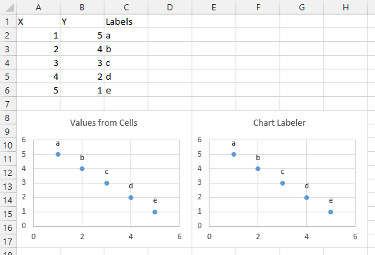
How to create Custom Data Labels in Excel Charts - Efficiency 365 Two ways to do it. Click on the Plus sign next to the chart and choose the Data Labels option. We do NOT want the data to be shown. To customize it, click on the arrow next to Data Labels and choose More Options … Unselect the Value option and select the Value from Cells option. Choose the third column (without the heading) as the range. How to Change Axis Values in Excel | Excelchat Right-click on the chart and choose Select Data Click on the button Switch Row/Column and press OK Figure 11. Switch x and y axis As a result, switches x and y axis and each store represent one series: Figure 12. How to swap x and y axis The chart will have more logic if we track store values per years. Create Dynamic Chart Data Labels with Slicers - Excel Campus You basically need to select a label series, then press the Value from Cells button in the Format Data Labels menu. Then select the range that contains the metrics for that series. Click to Enlarge Repeat this step for each series in the chart. If you are using Excel 2010 or earlier the chart will look like the following when you open the file. How to Create a Quadrant Chart in Excel – Automate Excel Step #9: Add the default data labels. We’re almost done. It’s time to add the data labels to the chart. Right-click any data marker (any dot) and click “Add Data Labels.” Step #10: Replace the default data labels with custom ones. Link the dots on the chart to the corresponding marketing channel names.
Excel Custom Chart Labels • My Online Training Hub Step 1: Select cells A26:D38 and insert a column Chart. Step 2: Select the Max series and plot it on the Secondary Axis: double click the Max series > Format Data Series > Secondary Axis: Step 3: Insert labels on the Max series: right-click series > Add Data Labels: Step 4: Change the horizontal category axis for the Max series: right-click ... How to Use Cell Values for Excel Chart Labels - How-To Geek Select the chart, choose the "Chart Elements" option, click the "Data Labels" arrow, and then "More Options." Uncheck the "Value" box and check the "Value From Cells" box. Select cells C2:C6 to use for the data label range and then click the "OK" button. The values from these cells are now used for the chart data labels. Excel Chart not showing SOME X-axis labels - Super User Apr 05, 2017 · In Excel 2013, select the bar graph or line chart whose axis you're trying to fix. Right click on the chart, select "Format Chart Area..." from the pop up menu. A sidebar will appear on the right side of the screen. On the sidebar, click on "CHART OPTIONS" and select "Horizontal (Category) Axis" from the drop down menu. Add or remove data labels in a chart - support.microsoft.com Click Label Options and under Label Contains, pick the options you want. Use cell values as data labels You can use cell values as data labels for your chart. Right-click the data series or data label to display more data for, and then click Format Data Labels. Click Label Options and under Label Contains, select the Values From Cells checkbox.
Adding rich data labels to charts in Excel 2013 | Microsoft ...
How to change chart axis labels' font color and size in Excel? 1. Right click the axis where you will change all negative labels' font color, and select the Format Axis from the right-clicking menu. 2. Do one of below processes based on your Microsoft Excel version: (1) In Excel 2013's Format Axis pane, expand the Number group on the Axis Options tab, click the Category box and select Number from drop down ...
Change Horizontal Axis Values in Excel 2016 - AbsentData
Excel tutorial: How to customize axis labels Now let's customize the actual labels. Let's say we want to label these batches using the letters A though F. You won't find controls for overwriting text labels in the Format Task pane. Instead you'll need to open up the Select Data window. Here you'll see the horizontal axis labels listed on the right. Click the edit button to access the ...

Change the format of data labels in a chart
Custom Chart Data Labels In Excel With Formulas - How To Excel At Excel Follow the steps below to create the custom data labels. Select the chart label you want to change. In the formula-bar hit = (equals), select the cell reference containing your chart label's data. In this case, the first label is in cell E2. Finally, repeat for all your chart laebls.

Google Workspace Updates: New chart text and number ...
Change the plotting order of categories, values, or data series Under Chart Tools, on the Format tab, in the Current Selection group, click the arrow next to the Chart Elements box, and then click the chart element that you want to use. On the Format tab, in the Current Selection group, click Format Selection. In the Axis Options category, under Axis Options, select the Series in reverse order check box.
Apply Custom Data Labels to Charted Points - Peltier Tech
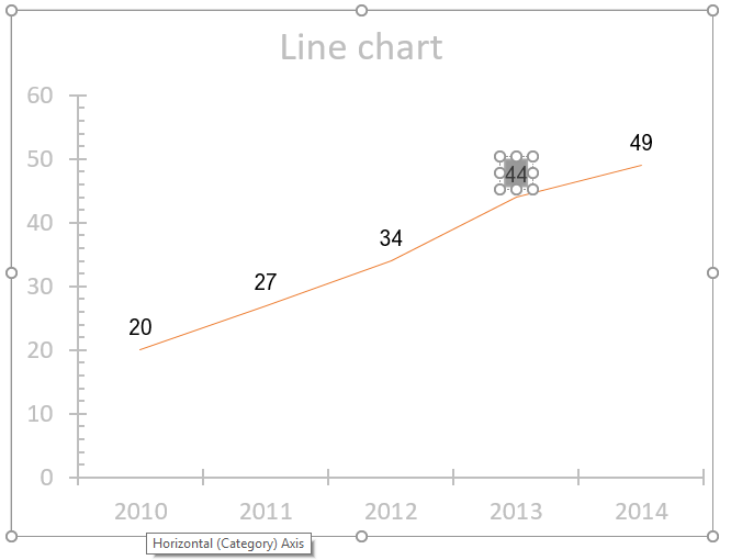
Edit titles or data labels in a chart - support.microsoft.com The first click selects the data labels for the whole data series, and the second click selects the individual data label. Right-click the data label, and then click Format Data Label or Format Data Labels. Click Label Options if it's not selected, and then select the Reset Label Text check box. Top of Page

How to use data labels in a chart
Use custom formats in an Excel chart's axis and data labels Right-click the Axis area and choose Format Axis from the context menu. If you don't see Format Axis, right-click another spot. Choose Number in the left pane. (In Excel 2003, click the Number ...

How to hide zero data labels in chart in Excel?
How to Customize Your Excel Pivot Chart Data Labels - dummies If you want to label data markers with a category name, select the Category Name check box. To label the data markers with the underlying value, select the Value check box. In Excel 2007 and Excel 2010, the Data Labels command appears on the Layout tab. Also, the More Data Labels Options command displays a dialog box rather than a pane.

Change the format of data labels in a chart
Modify Excel Chart Data Range | CustomGuide Select the chart. Click the Design tab. Click the Select Data button. From the Select Data Source dialog box, select the data series you want to move. Click the Move Up or Move down button. Click OK . The chart is updated to display the new order of data, but the worksheet data remains unchanged.

Improve your X Y Scatter Chart with custom data labels
Excel Chart Data Labels-Modifying Orientation - Microsoft Community In reply to PaulaAB's post on September 13, 2016. Hi Paula, You can right click on the data label part then select Format Axis. Click on the Size & Properties tab then adjust the Text Direction or Custom Angle. Thanks,

How to Place Labels Directly Through Your Line Graph in ...
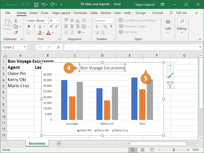
Excel charts: add title, customize chart axis, legend and data labels Select the chart and go to the Chart Tools tabs ( Design and Format) on the Excel ribbon. Right-click the chart element you would like to customize, and choose the corresponding item from the context menu. Use the chart customization buttons that appear in the top right corner of your Excel graph when you click on it.

Add or remove data labels in a chart
Change the format of data labels in a chart - Microsoft Support To get there, after adding your data labels, select the data label to format, and then click Chart Elements > Data Labels > More Options. To go to the appropriate area, click one of the four icons ( Fill & Line, Effects, Size & Properties ( Layout & Properties in Outlook or Word), or Label Options) shown here.

Custom Y-Axis Labels in Excel - PolicyViz
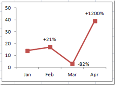
Percentage Change Chart – Excel – Automate Excel This tutorial will demonstrate how to create a Percentage Change Chart in all versions of Excel. Percentage Change – Free Template Download Download our free Percentage Template for Excel. Download Now Percentage Change Chart – Excel Starting with your Graph In this example, we’ll start with the graph that shows Revenue for the last 6…
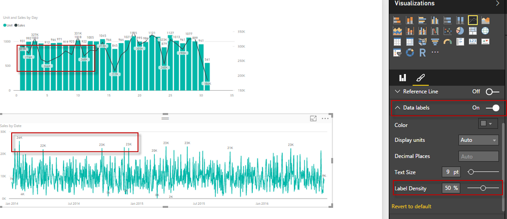
Solved: Data Labels - Microsoft Power BI Community
Excel Chart Vertical Axis Text Labels • My Online Training Hub Apr 14, 2015 · So all we need to do is get that bar chart into our line chart, align the labels to the line chart and then hide the bars. We’ll do this with a dummy series: Copy cells G4:H10 (note row 5 is intentionally blank) > CTRL+C to copy the cells > select the chart > CTRL+V to paste the dummy data into the chart.

Apply Custom Data Labels to Charted Points - Peltier Tech
excel - How do I update the data label of a chart? - Stack Overflow To build your data labels, somewhere else on your worksheet (conveniently, in the adjacent column would be ideal), use Excel formula to build the desired label string, for example: ="Blue occupies "&TEXT(B3,"0%") Repeat for the other points in the chart. Once you've done that, here's how you link Data Labels to a cell reference (normally, Data ...

Custom data labels in a chart
Custom data labels in a chart - Get Digital Help Press with mouse on "Add Data Labels". Press with mouse on Add Data Labels". Double press with left mouse button on any data label to expand the "Format Data Series" pane. Enable checkbox "Value from cells". A small dialog box prompts for a cell range containing the values you want to use a s data labels.
How to Edit a Legend in Excel | CustomGuide
How to format axis labels as thousands/millions in Excel? - ExtendOffice Right click at the axis you want to format its labels as thousands/millions, select Format Axisin the context menu. 2. In the Format Axisdialog/pane, click Number tab, then in theCategorylist box, select Custom, and type[>999999] #,,"M";#,"K"into Format Codetext box, and click Addbutton to add it toTypelist. See screenshot: 3.

Custom Excel Chart Label Positions • My Online Training Hub
Custom Data Labels with Colors and Symbols in Excel Charts - [How To ... To apply custom format on data labels inside charts via custom number formatting, the data labels must be based on values. You have several options like series name, value from cells, category name. But it has to be values otherwise colors won't appear. Symbols issue is quite beyond me.

Apply Custom Data Labels to Charted Points - Peltier Tech
How to Change Excel Chart Data Labels to Custom Values? May 05, 2010 · First add data labels to the chart (Layout Ribbon > Data Labels) Define the new data label values in a bunch of cells, like this: Now, click on any data label. This will select “all” data labels. Now click once again. At this point excel will select only one data label.

How to hide zero data labels in chart in Excel?
Multiple Time Series in an Excel Chart - Peltier Tech Aug 12, 2016 · Start by selecting the monthly data set, and inserting a line chart. Excel has detected the dates and applied a Date Scale, with a spacing of 1 month and base units of 1 month (below left). Select and copy the weekly data set, select the chart, and use Paste Special to add the data to the chart (below right).

Apply Custom Data Labels to Charted Points - Peltier Tech

How-to Use Data Labels from a Range in an Excel Chart - Excel ...

Add or remove data labels in a chart
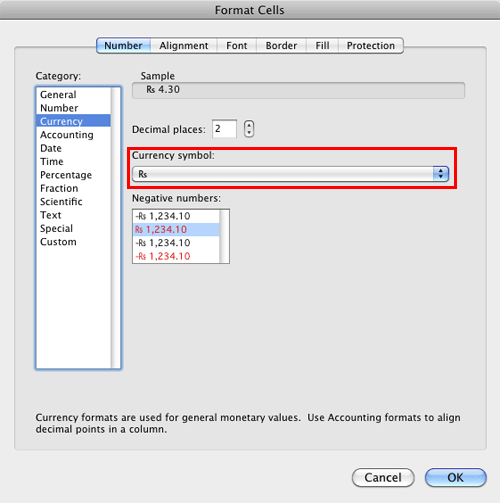
Format Number Options for Chart Data Labels in Excel 2011 for Mac
How-to Add Custom Labels that Dynamically Change in Excel ...

Apply Custom Data Labels to Charted Points - Peltier Tech

How to Add Data Labels to an Excel 2010 Chart - dummies

How to Add Axis Labels to a Chart in Excel | CustomGuide

Change color of data label placed, using the 'best fit ...

Custom Data Labels with Colors and Symbols in Excel Charts ...

Dynamically Label Excel Chart Series Lines • My Online ...

Add Labels ON Your Bars

Change the format of data labels in a chart

Format Data Labels in Excel- Instructions - TeachUcomp, Inc.

Custom Data Labels with Colors and Symbols in Excel Charts ...
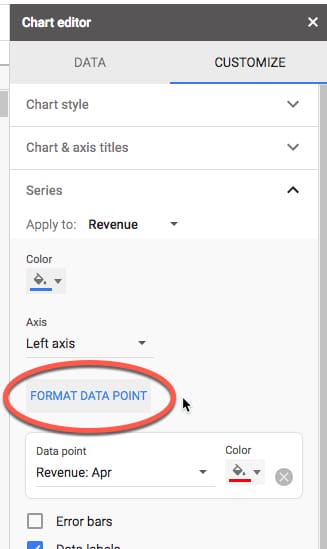
How can I format individual data points in Google Sheets ...

How can I hide 0% value in data labels in an Excel Bar Chart ...

Excel sunburst chart: Some labels missing - Stack Overflow

Google Workspace Updates: Get more control over chart data ...
How to add and customize chart data labels

Using the CONCAT function to create custom data labels for an ...

Excel charts: add title, customize chart axis, legend and ...
Post a Comment for "41 how to change excel chart data labels to custom values"